Grad School Scramble I: Ordinary Least Squares Estimation

I am proud to announce that I will be attending ASU in the fall to pursue a PhD in quantitative psychology under the guidance of Kevin Grimm! This decision was arrived at after a long and arduous application process wherein I flew to 7 different programs to interview. After all of my traveling, ASU was the one that felt most like home.

To prepare for grad school, I figured that it would be helpful and cathartic (and a little bit exposing) to use the blog to revisit some of the beginner topics in quantitative psychology that I am not incredibly well-versed in. Thus: Welcome to the birth of Grad School Scramble!!! In each installment of this multi-part series, I will attempt to learn and explain some area, subject, or topic of quantitative psychology that I had previously not understood well. Important disclaimer: this is a judgement-free zone! If I cover some concept that makes you say, “Hey, shouldn’t an incoming PhD student have a better understanding of this subject matter?” then, well, too bad! In this pastel-gray and baby-blue blog page, we can all find solace together in the fact that we are amateurs.

Today’s topic: Ordinary Least Squares Estimation in Linear Regression (And Other Methods)

Kevin has been doing this awesome thing where he sends me small coding assignments designed to introduce me to the field of data simulation in advance of my first semester. These assignments are typically in R, and they normally involve me simulating some data on which I perform some statistical technique. For the first one, here was the task: Generate $n=500$ where $x_{1i}$ follows a standard normal distribution (mean = 0, std = 1), and $y_i=.5⋅x_{1i}+e_i$ where $e_i$ is normally distributed with a mean of 0 and a variance of .75. It was a nice little foray into data simulation, and I also calculated an estimated slope coefficient each time the data were generated.

However, this got me thinking. To determine the coefficient I used the lm function, which states the following as one of its parameters:

weights

an optional vector of weights to be used in the fitting process. Should be NULL or a numeric vector. If non-NULL, weighted least squares is used with weights weights (that is, minimizing sum(w*e^2)); otherwise ordinary least squares is used.

Notice that? Ordinary least squares. I realized that I didn’t actually have a good handle on what the ordinary least squares estimation method was doing, so I spent some time googling it.

Background

To contextualize, let’s get a quick run-down on linear regression. (Feel free to skip this entire section if you are familiar with it.)

Linear regression, at its core, aims to estimate the level of some outcome variable, say $y$, on the level of some predictor variable, say $x$. Imagine that you have some (ambiguous) set of data like so:

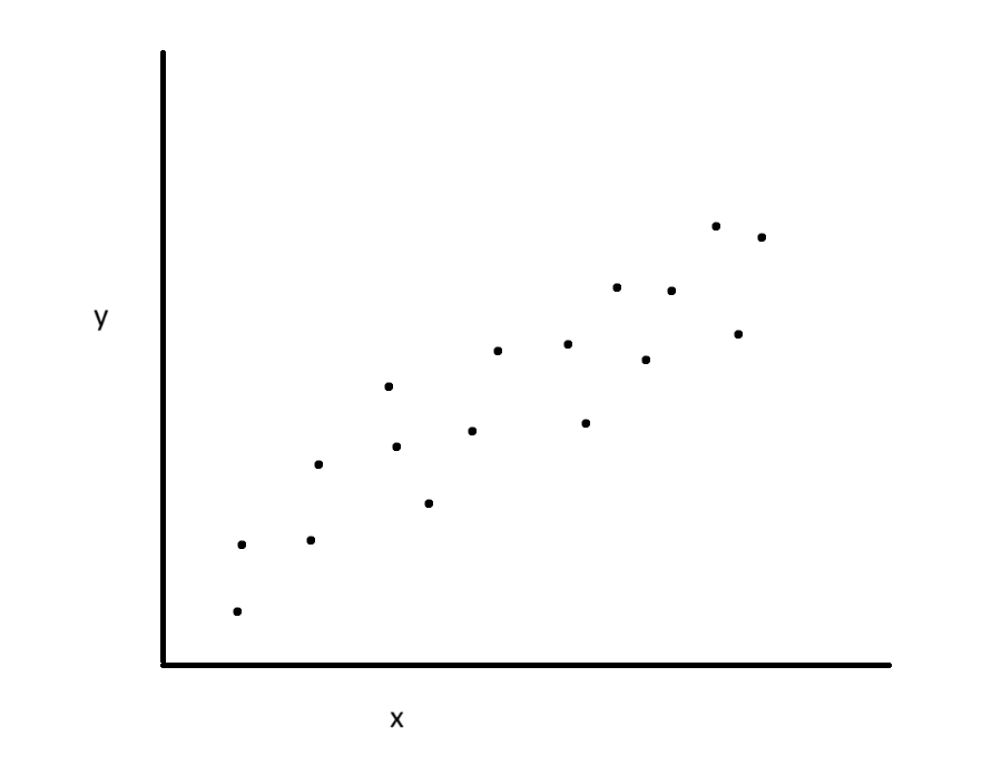
You might rightly notice that there is a general relationship between variable $x$ and variable $y$: as the level of $x$ increases, so does $y$ (generally). You then might ask: is there a way, given $x$, to predict a corresponding value for $y$? This is exactly what linear regression aims to do—to create a non-deterministic formula which predicts outcomes from a given predictor. One way to do this is by fitting a line (linear regression) that follows the trend of the data:

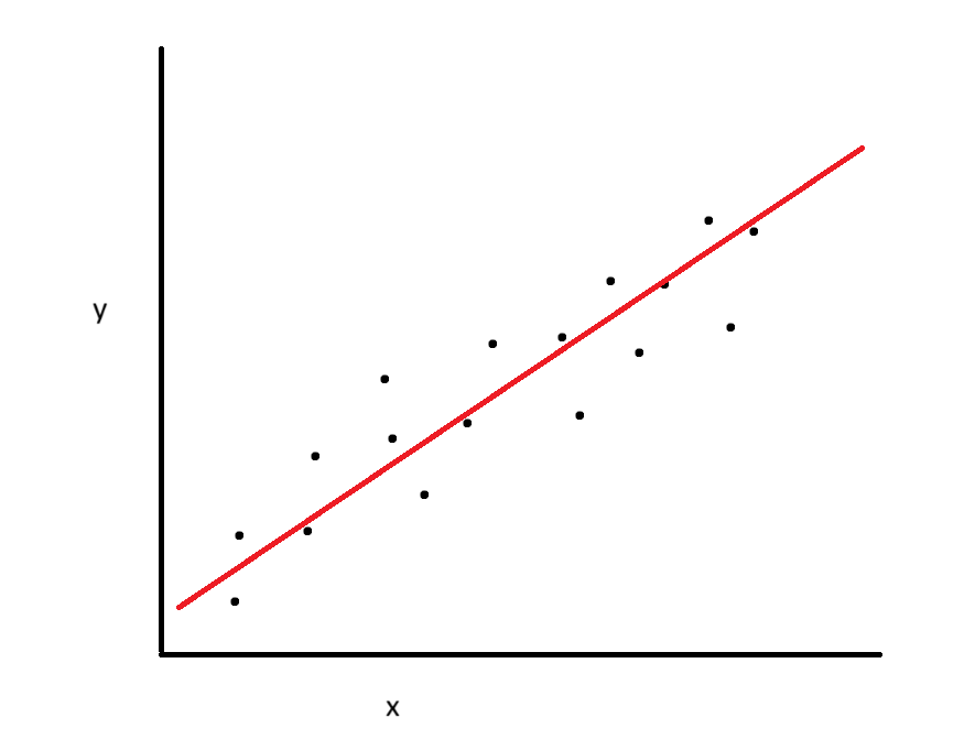
As per our 8th grade math education, we know that this line would take the form of $y=mx+b$, where $m$ is the slope and $b$ is the intercept. If our line perfectly described the data, then we would be able to perfectly predict each level of $y$ from each observation of $x$. Unfortunately, as we can see from the fact that not all of our data points fall along the line, it is not a perfect prediction. We call this error, or the residuals. So, linear regression aims to incorporate this by adding a third variable to the equation of the line: the variance of the residuals. Let’s dissect this.

Generally, when we fit the line to the data, we expect the data points to be closer to the line than away from it. For the purposes of linear regression, we assume that they do so in a normal manner. Thus, for each level of the $x$ variable, there is a range of values we would expect for the $y$ variable.

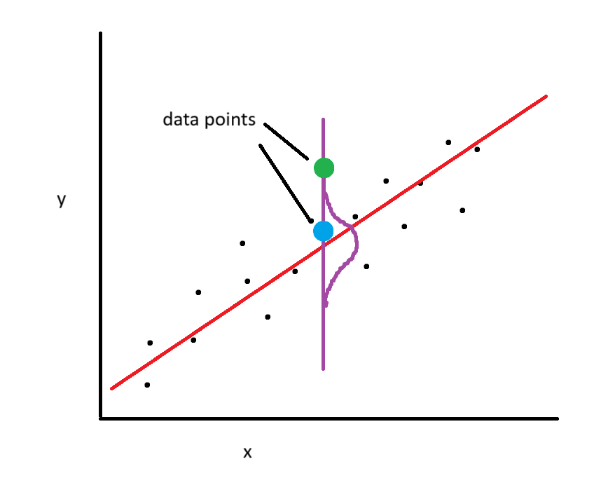
For example, in this picture the purple curve shows the range of values we would expect from $y$ at the given point. We would expect to see the blue dot more than we would expect to see the green dot. (This assumption is called the assumption of normality of the residuals and the assumption that this range is the same at all levels is homoscedasticity.)

Regression accounts for this in the following manner: If we want to predict $Y$, we can do so by predicting it from two measures—a function of $X$, and an error term $ε$. If our function of $X$ is linear, we get the following form:

$Y_i=β_0+β_1X_i+ε_i$

where $β_1$ is basically the $m$ and $β_0$ is basically the $b$ in $y=mx+b$. The “spread” of data around the line is accounted for by $ε$.

We tracking so far? Basically, once we have values for $β_0$ and $β_1$ and understand our error, we can regress $y$ on $x$ to understand their relation.

Ordinary Least Squares Estimation Theory

The question then becomes: how do we estimate values for $β_0$ and $β_1$? Think back to our previous (data-ambiguous) example. If you wanted to draw a “line of best fit” through the data, you might come up with the line we drew previously:

However, maybe your colleague disagrees, and says that a different line (orange) actually fits the data better:

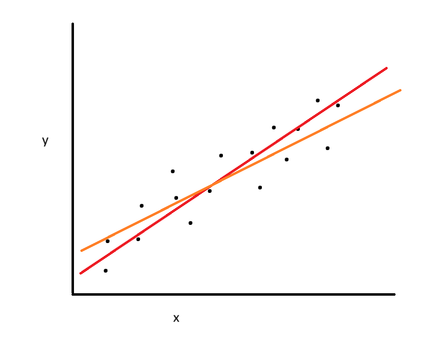
We need to come up with some objective way to state that a line fits the data best. This is where Ordinary Least Squares Estimation comes in. One way to objectively state that a line fits “best” is to attempt to minimize the distance between each data point and the line of prediction. Recall that the distance is defined as the error:

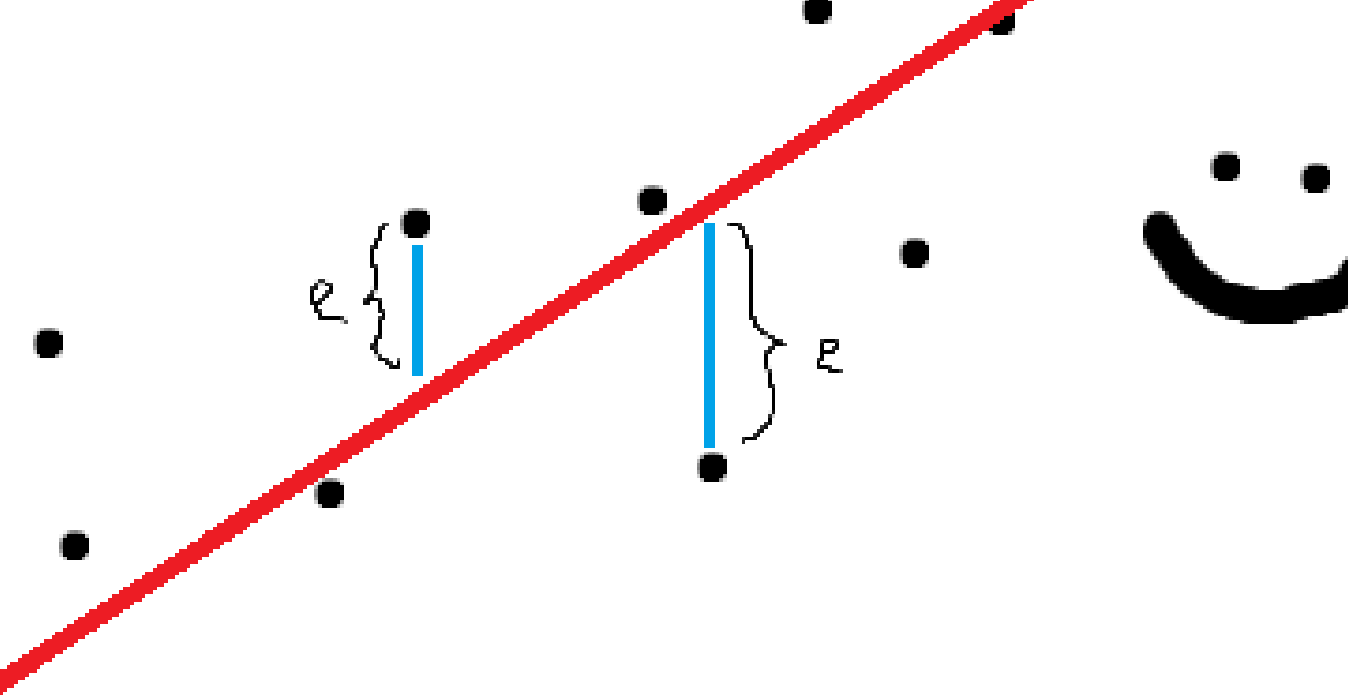
If our line fits reasonably well, we would expect the distance between the points and the line to be small. For a counterexample, a terrible line of prediction:

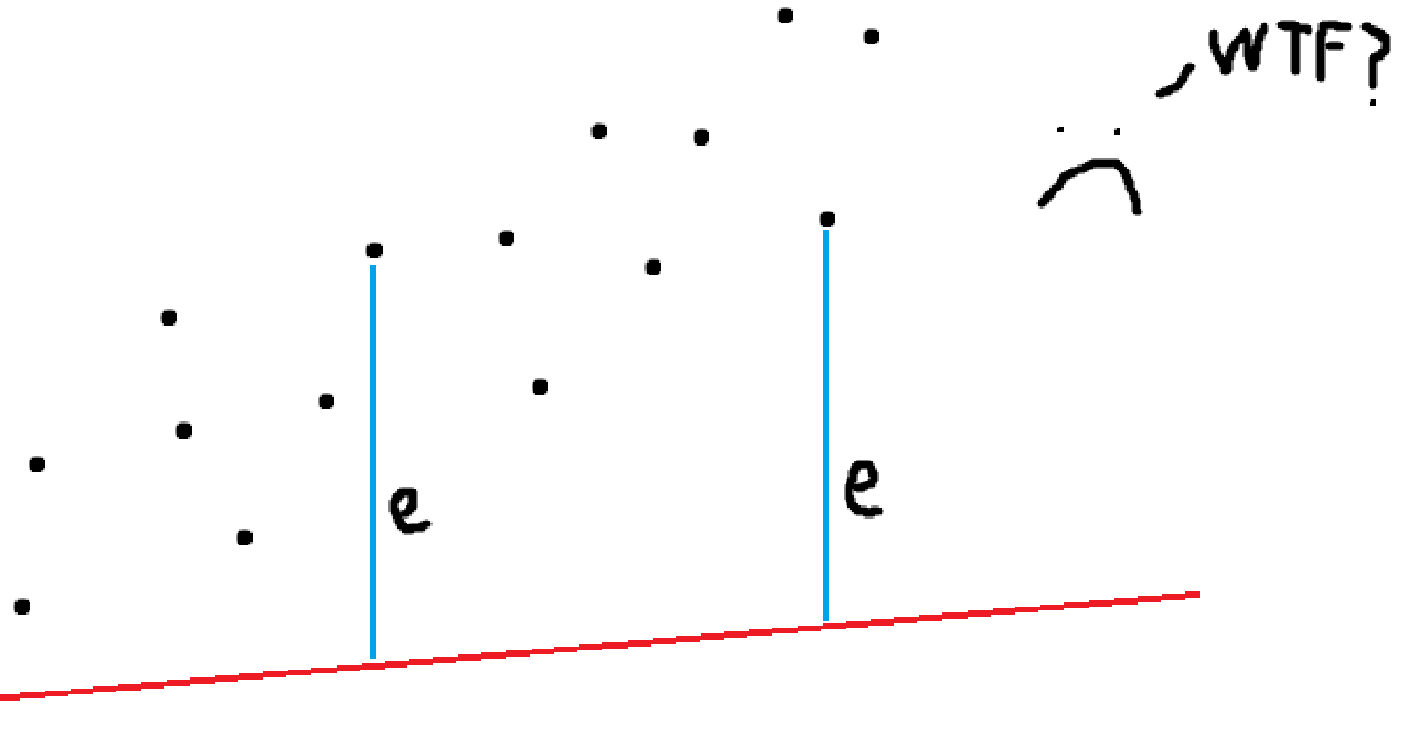
See how big the distance (error) is? This is the basis of Ordinary Least Squares: the smaller the overall error, the better.

Soooo… this is easy, right? Just minimize the total amount of error! Well, there’s one problem. If we have a large positive distance between a point and the line, and we have a large negative distance between another point and the line, they cancel out, and the overall error is 0. So, we instead square the distances so that we can meaningfully compare them. If we can find values for $β_0$ and $β_1$ that minimize the squared error, we have our line.

Ordinary Least Squares Estimation Calculation

All the previous description of linear regression was assuming that we knew population values for our data. In reality, we always work with samples. So, we transform our previous population equation $Y_i=β_0+β_1X_i+ε_i$ to a sample-specific equation:

$y=b_0+b_1x+e$.

Well, we might notice something. In this equation, $y$ is the actual data point that we observe. But we also have access to another version of $y$: $ŷ$. This symbol represents the predicted value of $y$ for a given data point—the value for $y$ we would expect without error. Thus, we also have the equation $ŷ=b_0+b_1x$ by definition.

Yay! Now we can do some algebra.

$y=b_0+b_1x+e$ and $ŷ=b_0+b_1x$. Thus,

$y=ŷ+e$

$e=y-ŷ$

Well now! Recall that we’re trying to minimize the residuals for our line of prediction. Now we have a definition for them. According to our previous theory, we need to square this term to meaningfully compare observations:

$e^2=(y-ŷ)^2$

And all we need to do is sum these babies up and find the values for $b_0$ and $b_1$ that minimize that sum!

$∑(y-ŷ)^2$

Example: Ordinary Least Squares Estimation with Three Data Points

Let’s illustrate this calculation with an example (which I came up with myself, so bear with me). Imagine that we have 3 data points, and we want to estimate the slope and intercept of a prediction line via our previously-discussed method. We’ll say these points are $(1,2)$, $(2,3)$, and $(4,6)$.

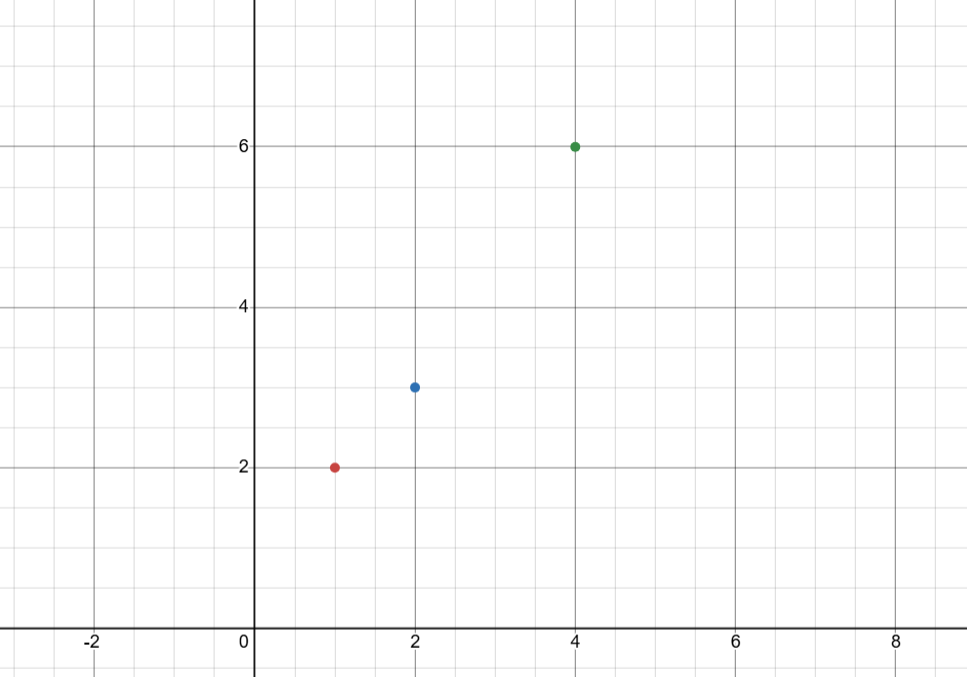
Recall our previous formulae: $y=b_0+b_1x+e$ and $ŷ=b_0+b_1x$. We want to solve for the values of $b_0$ and $b_1$ by minimizing the sum $∑(y-ŷ)^2$. So, let’s use some calculus.

How can we find the local minimum of a function? By calculating its derivative and determining when the derivative is equal to $0$. Remember, the derivative of a function at a certain point represents the rate of change of the function at that point: in other words, the slope of the tangent line at that point. So, if we know that the slope of the tangent line is $0$ (and that we’re looking for a minimum), we know that the function is going from decreasing to increasing, and we have found a local minimum.

So, let’s calculate the sum $∑(y-ŷ)^2$ and find its derivative!

$∑(y-ŷ)^2$ will have 3 different components: one for each point. Let’s label these $(y_1-ŷ_1)^2$, $(y_2-ŷ_2)^2$, and $(y_3-ŷ_3)^2$ where $point 1 = (1,2)$, $point 2 = (2,3)$, and $point 1 = (4,6)$.

Remember, $ŷ=b_0+b_1x$. So for each observation we can plug the actual point’s value of $y$ in for $y_i$ and plug in our variables of $b_0$ and $b_1$ for $ŷ_i$. This will let us get a function in terms of $b_0$ and $b_1$—the values we want to solve for.

$(y_1-ŷ_1)^2=(2-(b_1+b_0))^2$

$(y_2-ŷ_2)^2=(3-(2b_1+b_0))^2$

$(y_3-ŷ_3)^2=(6-(4b_1+b_0))^2$

In each equation, we put the x-value of the point alongside the variable $b_1$ because our predicted value $ŷ$ is a function of $b_0+b_1x$.

Now, we mash all of these components together:

$∑(y-ŷ)^2=(2-(b_1+b_0))^2+(3-(2b_1+b_0))^2+(6-(4b_1+b_0))^2$

Next is finding the derivative. Let’s expand this equation so we’re not dealing with exponents around parentheses (I’m gonna gloss over a few intermediate steps).

$∑(y-ŷ)^2=4-4b_1-4b_0+b_1^2+2b_1b_0+b_0^2+9-12b_1-6b_0+4b_1^2+4b_1b_0+b_0^2+36-48b_1-12b_0+16b_1^2+8b_1b_0+b_0$

$∑(y-ŷ)^2=21b_1^2-64b_1+3b_0^2-22b_0+14b_1b_0+49$

Awesome! Now we have a more manageable function with two variables. We want to find the minimum of this function with respect to both, so we take the partial derivative with respect to $b_1$ and $b_0$. (Again, skipping some intermediate steps.)

$\frac{d}{db_1}=42b_1-64+14b_0$

$\frac{d}{db_0}=6b_0-22+14b_1$

Ok. Home stretch. Now we set these two equations equal to 0:

$42b_1-64+14b_0=0$, and $6b_0-22+14b_1=0$. We can set up a system of equations:

$42b_1+14b_0-64=0$

$14b_1+6b_0-22=0$

Which we can actually transform into a matrix by putting the constants on the right-side of the equation:

$\overset{3r_2}{\longrightarrow}$

$\overset{r_2-r_1}{\longrightarrow}$

So, the solution to the system of equations which sets both derivatives equal to 0 includes $b_0=\frac{1}{2}$. We can plug this value into the first equation to obtain:

$42b_1+14(\frac{1}{2})-64=0$

$42b_1+7-64=0$

$42b_1-57=0$

$42b_1=57$

$b_1=\frac{57}{42}$

$b_1=\frac{19}{14}$

You get to see all the steps that time. Well, OK! Now we know the values for which our function $∑(y-ŷ)^2$ has a local minimum! So, if our calculations are correct, we should be able to plug those values back into the formula $y=b_0+b_1x+e$ to obtain a slope and intercept coefficient for our regression.

Let’s try it:

$y=\frac{1}{2}+\frac{19}{14}x$:

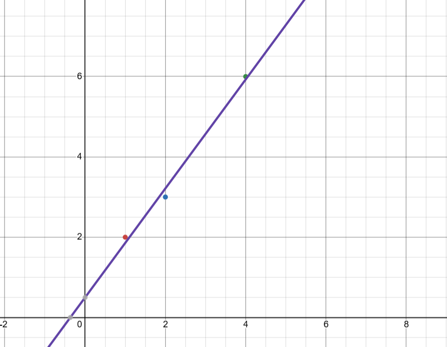
Hey that looks pretty good! Like, really good! I made the starting numbers up on the fly, so I’m happy to see that we got an equation with nice simple fractions and not complex decimals.

The final part of calculating the linear regression is to get the variance of the residuals (I’m gonna speed through this). Using our formula for variance we can see that $\hat{σ}^2=\frac{1}{n-p}∑\hat{ε_i}^2$ where we divide by $n-p$ as the number of degrees of freedom for $p$ parameters. We can recall that $\hat{ε_i}=y_i-ŷ_i$ by definition, and use our new slope and intercept to calculate $ŷ$ for each observation.

For $(1,2)$:

$y-ŷ=2-ŷ=2-(\frac{1}{2}+\frac{19}{14}(1))\approx0.143$

For $(2,3)$:

$y-ŷ=3-ŷ=3-(\frac{1}{2}+\frac{19}{14}(2))\approx-0.214$

For $(4,6)$:

$y-ŷ=6-ŷ=6-(\frac{1}{2}+\frac{19}{14}(4))\approx0.071$

We can sum the squares of these $3$ values: $(.143)^{2}+(-.214)^{2}+(.071)^{2}\approx0.071$.

Finally, we divide this value by $n-p=3-2=1$. Dividing by $1$ does not change the number, and so our $\hat{σ}^2=0.071$.

So, all together, we have the following formula for our linear model: $y=\frac{1}{2}+\frac{19}{14}x+e$ with $\hat{σ}^2=0.071$.

Verification

Let’s see how we did. Here is code which runs it in R:

x <- c(1, 2, 4)

y <- c(2, 3, 6)

d <- lm(y~x)

summary(d)

(summary(d)$sigma)**2

And here is the output:

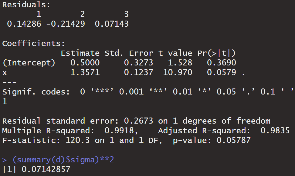
Holy mackerel. That looks great. Notice that under “Coefficients” we can see the estimate for the intercept at $0.5000$, which is exactly what we predicted. Similarly, the estimate for the slope is $1.3571$, which is approx. $\frac{19}{14}$. Spot on.

Also, notice the residuals: $0.14$, $-0.21$, $0.07$. Do those numbers look familiar? Finally, we can observe the sigma**2 value at the end, and notice that it is incredibly close to the value we predicted of $0.071$.

WE DID IT!!!!!!!!

Conclusion

So there you have it. How to hand calculate ordinary least squares estimation in a linear regression. Much like all my blog posts, this ran on far longer than I originally meant it to. Congrats if you stuck around till the end. For the next installment of Grad School Scramble, I’ll try to keep it more theoretical and less concrete. I don’t like wrangling $\LaTeX$.