Recently, I woke up to a phone call from my grandfather asking me to explain the Monty Hall Problem in simple terms. For those of you who are unfamiliar, this problem is famous in the field of probability for confounding even highly-training individuals (like mathematicians and academics) due to its unintuitive nature.

The problem is thus: Imagine that you’re on a TV show, and the host asks you to pick randomly from three doors. Behind two of the doors is a goat, and behind one of the doors is a brand-spanking-new car. After you select one of the doors, the host then intentionally selects one of the other doors to reveal a goat. He then asks if you want to switch your guess to the other door or stay on your current guess. Is it to your advantage to switch?
Many people say that it doesn’t matter: your choice is a 50/50 between your door having a goat or a car. However, the true solution is that it is definitely to your advantage to switch! Swapping doors gives you a 2/3 chance to win the car.
The reason for this has a lot to do with probability theory and other unintuitive math, but it boils down to the idea that if you started off picking a goat, you’ll win the car by swapping after the host reveals the other goat. Only if you start on the car would swapping win you a goat. You can also consider the three different possibilities in the chart below:
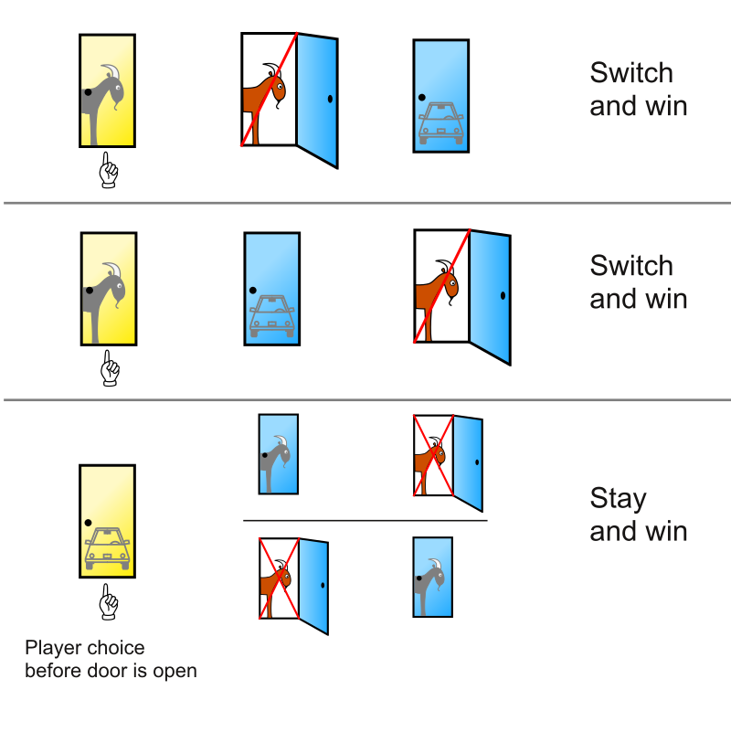
As we can see, 2/3 scenarios win the car by swapping.
After (unsuccessfully) trying to explain this to my grandfather and other family, it got me thinking about the topic of probability in general. I have actually never taken a probability course, and it’s one of the areas of quantitative methodology that I’m probably weakest in. So, I figured that it would be a good idea to get a basic intro to some of the ideas in probability theory. Thus the second installment of Grad School Scramble™ was born.
Preparation
To see what topics I didn’t already have a good grasp of, I took an open-source final from an MIT probability course and graded myself using the provided key. Holy smokes, I have a long way to go. I had a solid understanding of most of the counting/set theory stuff just because I have taken a course on discrete mathematics, but most of the other material I was lost on. After my self-confidence was ground into pieces, I realized that a blog post covering an entire probability course was probably unfeasible, so I came up with a list of easier concepts to learn (and saved the multivariate calculus stuff for another time).
Conditional Probability
Conditional probability was the first concept that I didn’t have much prior experience with. I had worked with various concepts related to probability and counting in my discrete math course, including the principle of inclusion/exclusion and different methods of counting with combination/permutation rules. However, we never explicitly forayed into the world of conditional probability.
At its core, the idea of conditional probability answers the question “how does the likelihood of an event change given additional information?” When I was first reading about it, my intuition told me that you could answer this question with simple counting techniques: for example, what is the probability of a card from a standard deck having a suit of hearts given that its color is red? It seemed as if you could simply use logic to determine the sample space (red heart, red diamond, black club, black spade) and only use the subset containing the necessary event. However, this method is a bit constrained and only applicable for simple problems.
A formal definition of conditional probability is as follows:
$P(A\mid B)=\frac{P(A\cap B)}{P(B)}$
This reads as “the probability of $A$ given $B$ is equal to the probability of $A$ and $B$ divided by the probability of $B$.”
I had never seen this formula before. Intuitively, it makes sense, though. If $A$ and $B$ are dependent events, then dividing out the probability of $B$ from the intersection of $A$ and $B$ seems to leave you with only the probability of $A$ (given that $B$ has already occurred).
Another way to interpret this is by considering venn diagrams.
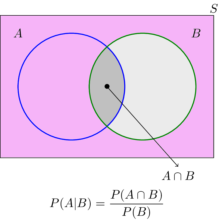
When we state that $B$ has already occurred, we can discard the entire region outside of $B$ (everything in pink). Thus, we are left with $\frac{P(A\cap B)}{P(B)}$ as the total probability of $A$ occurring.
One important consideration to make is that we can rewrite the formula as $P(A\mid B)P(B)=P(A\cap B)$ by simple multiplication. Thus, if we know the conditional probability of something we can use this formula to find the probability of event intersections.
Let’s use this formula to solve a problem. Approximately 10% of cars are red. What is the probability that two red cars get into an accident on the highway given that one of the cars is red? We can define $P(A)$ as the probability that the crash has two red cars and $P(B)$ as the probability that at least one car is red. Because $A$ is necessarily a subset of $B$ (for both cars to be red, at least one must be red), we can see that $P(A\cap B)=A=.01$. $P(B)$ is the complement of neither car being red, so $P(B)=1-(.9\cdot.9)=.19$. Because $\frac{.01}{.19}\approx.053$, the overall probability $P(A\mid B)\approx.053$.
It seems a bit counterintuitive that the answer isn’t just $.1$. After all, it seems like we know one of the cars is red, so the probability of the other car being red as well should just be $.1$. However, we don’t specifically know which car is red. Imagine that we specify the cars as Car 1 and Car 2. Our event space is as follows (for $R=red$ and $N=not red$): ${(R,N), (N,R), (R,R), (N,N)}$. When we use the logic of “one of the cars is red, so the probability of the other one being red as well should just be $.1$”, we implicitly make the assumption that we’re talking about Car 1 being the red one. However, the event that at least one of the cars is red comprises the set ${(R,N), (N,R), (R,R)}$ while the event that Car 1 is red comprises ${(R,N),(R,R)}$. Because $(N,R)$ is non-empty (we know that it could be the case that Car 2 is the red one), we know that the probability of both cars being red is smaller when we only know one car is red compared to when we know Car 1 is red (because in the first scenario $(R,R)$ is selected from a larger event space than in the second).
Another note: Two events can be considered formally independent if $P(A\mid B)=P(A)$. This is because they are independent if knowing that $B$ has occurred does not change the probability of $A$. It then follows that if two events are independent then $P(A\cap B)=P(A\mid B)\cdot P(B)=P(A)\cdot P(B)$, which follows our prior understanding of probability.
Bayes’ Theorem
Throughout the murky, dark waters of statistics and probability, one beast lies dormant, slumbering, waiting for an unfortunate soul to stumble across its gaping maw. This beast is none other than Bayes’ Theorem, striking fear into the hearts of frequentists everywhere (before you write an angry email—I know that Bayes’ Theorem itself is not wholly relegated to Bayesian statistics).
Much like conditional probability, I hadn’t much experience with Bayes’ Theorem before looking into it. In one of my undergraduate psych classes with Dr. Terry, we discussed the famous Kahneman and Tversky base rate fallacy in terms of Bayes’ Theorem: where individuals fail to incorporate the base rate of an event and obtain incorrect probabilistic deductions. Here is the theorem in all its glory:
$P(A\mid B)=\frac{P(B\mid A)\cdot P(A)}{P(B)}$.
This theorem lets us find the inverse of a conditional probability: If we know the probability of $A$ given $B$, we can now find the probability of $B$ given $A$. The proof follows from our previous conditional probability formula:
$P(A\cap B)$ is symmetric with respect to $A$ and $B$, so
$P(B\mid A)\cdot P(A)=P(A\cap B)=P(A\mid B)\cdot P(B)$.
Then, if we divide by $P(A)$ we obtain Bayes’ Theorem.
We can use this tool to answer the Monty Hall problem discussed earlier. If event $A$ is that the car is behind our door (door 1), and event $B$ is that the host opened door 3, we find the probabilities and substitute them in:
$P(B\mid A)$ will be $.5$ because the probability of the host opening door 3 given that the car is behind our door is $.5$ (he could have chosen either door 2 or door 3).
$P(A)=\frac{1}{3}$
$P(B)=.5$ (There are three scenarios: the car is behind our door, which gives Monty a .5 probability of picking door 3, the car is behind door 2, which gives Monty a 1 probability of picking door 3, and the car is behind door 3, which gives Monty a 0 probability of picking door 3. Thus, the total probability [$(.5 + 1 + 0) * \frac{1}{3}$] of Monty picking door 3 is .5)
So:
$P(A\mid B)=\frac{.5 \cdot \frac{1}{3}}{.5}=\frac{1}{3}$.
In other words, the probability of the car being behind our door given that Monty opened door 3 is $\frac{1}{3}$. Thus, it is in our interest to switch doors.
Bayes’ Theorem can also be stated as $Posterior=Prior \cdot Likelihood$, where each part of the statement is part of our original formula.
Common (Discrete) Probability Distributions
Next, I’d like to cover a few distributions that I was a little shaky on. It’s easy to fixate on the normal distribution as the “big one” of important distributions, but many data-generating processes are non-normal. Also, this gave me a chance to practice my plot-making skills in R.
For discrete distributions (which all of the following distributions are), the probability mass function, or pmf, is the function which gives the probability of a random variable from the distribution being equal to a given variable. This function is written $p(a)$ where $a$ is the variable of interest. This will be important as we examine different distributions.
Bernoulli Distribution
The Bernoulli distribution is a simple one: it models one trial in an event with a binary outcome. So, for example, if we’re observationally assessing the behavior of dogs being walked in a park (and want to determine whether or not they will urinate on a fire hydrant), the behavior of one specific dog would be modeled by a Bernoulli distribution.
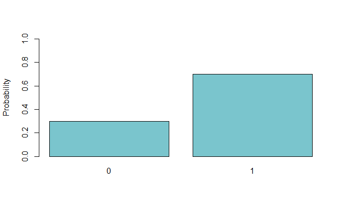
The Bernoulli distribution takes one parameter, $p$, which represents the underlying probability of a $1$ for the outcome. If 70% of dogs will pee on the fire hydrant, then $p=.7$. If $X$ is the variable of interest, by definition $P(X=1)=p$.
Here’s an example of a Bernoulli distribution with $p=.7$:
Binomial Distribution
The binomial distribution is an extension of the Bernoulli distribution. It models the probability of an event (binary, represented by a Bernoulli distribution) occurring a certain number of times in a set number of trials. It has two parameters: $n$ (the number of trials) and $p$ (the probability of a success).
For example, if we wanted to determine the probability of flipping a certain number of heads in ten total flips of a coin, we might use the following binomial distribution:
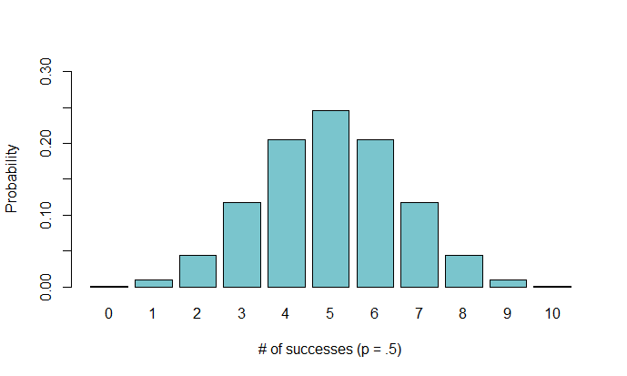
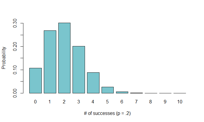
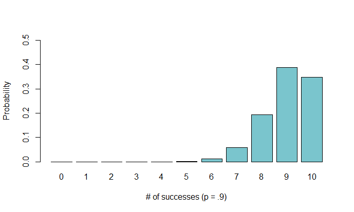
By looking at this distribution, we can see the approximate probability of flipping a certain number of heads out of 10 flips with a fair coin ($p=.5$). For example, the chance of flipping exactly 3 heads is around $12\%$. It looks Gaussian, but this is only because our probability of a heads is $.5$. If we want to imagine that the coin we are flipping is unfair, we can assess the following distributions with $p=.2$ and $p=.9$, respectively:
How do we obtain these distributions? The pmf for a binomial distribution with probability $p$ and # of trials $n$ is defined as
$P(X=k)=\binom{n}{k}p^k(1-p)^{n-k}$
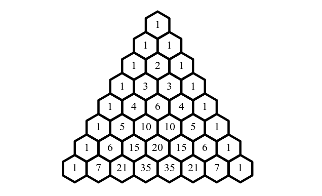
From this, we can see why it’s called the binomial distribution. The $n$ choose $k$ part of the formula is a binomial coefficient: coefficients of binomial expansion that follow Pascal’s Triangle.
Geometric Distribution
Geometric distributions model the probability of a certain number of failures before a success in a sequence of Bernoulli trials. In other words, they show how many tails you can expect to flip before you get a heads.
If $X$ is the number of tails, the pmf for a geometric distribution is defined as:
$P(X=k)=(1-p)^kp$
where $p$ is the probability of a success. The intuition behind this formula is that it’s simply a representation of the odds of getting the desired sequence. For example, if you want to find the odds of flipping 4 heads before a tails, you would find the odds of getting HHHHT, which is simply $.5^5$.
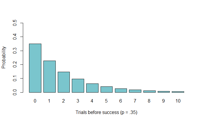
Take a look at the following distribution:
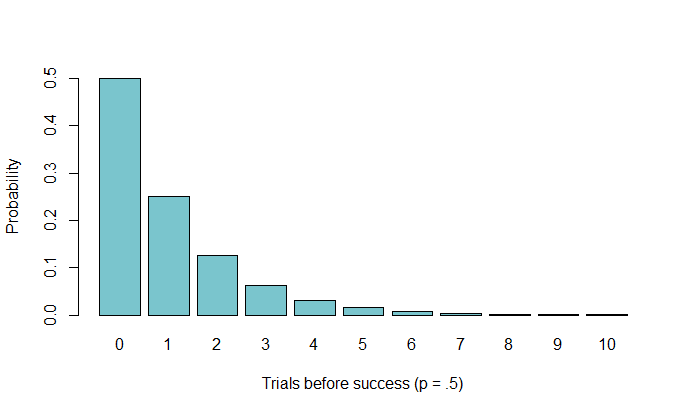
From this, we can see the probability behind each number of tails before getting a heads. The interpretation of $0$ is that the first flip was a heads. Again, if we were using an unfair coin, the distribution might look something like this:
Poisson Distribution
The Poisson distribution models the number of fish you can expect to catch in a given period of time. Just kidding. Kind of. This distribution was named after the French mathematician Simeon Poisson, whose last name translates to “Fish.” It models the expected number of events in a certain period of time given the average number of observed events. For example, if you know that you pass 3 gas stations every half-hour on a road trip, and you wanted to determine the probability of passing 5 in the next half-hour, you might use a Poisson distribution.
It has one parameter: $\lambda$. This paramter is the average number of successes for the specified time period. The pmf is defined as
$P(\lambda, k)=\frac{\lambda^ke^{-\lambda}}{k!}$
where $k$ is the desired number of successes per period.
We’ve officially passed into the realm of pmf’s that I don’t understand. Intuitively, you can derive this from the binomial distribution by setting up a formula which represents a number of discrete probability chunks, each with probability $\frac{\lambda}{n}$ (where $\lambda$ is the average # of events per time period and $n$ is the number of discrete chunks). A binomial distribution models the expected number of successes given a certain probability and number of trials, so we can substitute this probability into a binomial limit as $n\rightarrow \infty$. After some complicated math with limits and $e$, we get the pmf of a Poisson distribution.
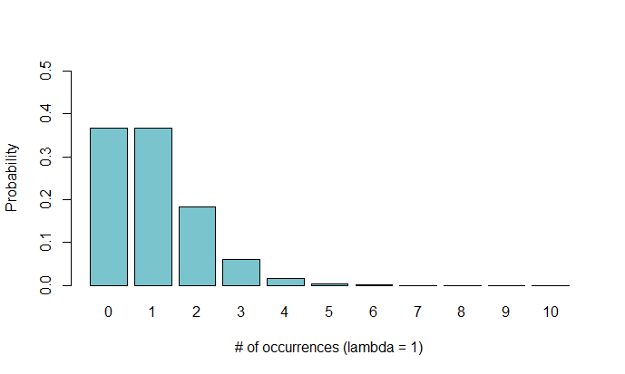
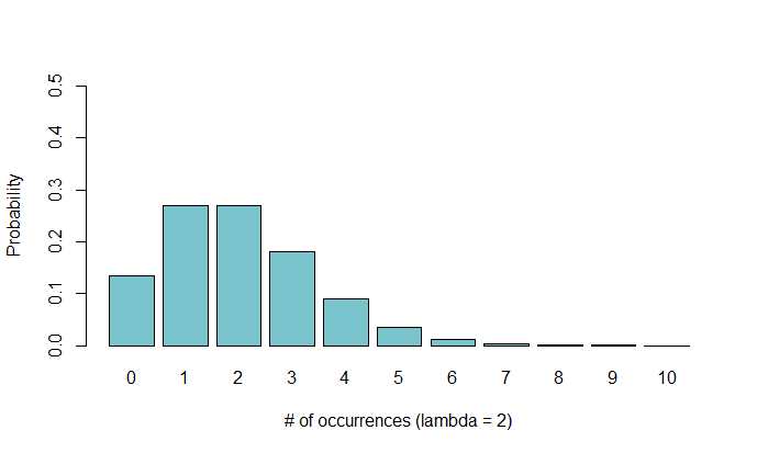
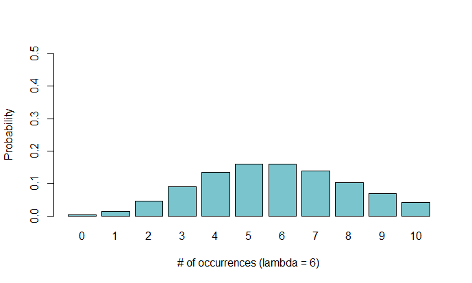
Below you can see a Poisson distribution for $\lambda=1$, $\lambda=2$, and $\lambda=6$.
Many of these discrete distributions have analogues in continuous distributions (for example, the geometric distribution and the exponential distribution). I chose not to cover the continuous distributions because I was already at least conceptually familiar with them, but maybe I’ll dive into their probability functions in a later post.
Concluding Thoughts
Well, that covers a lot of the things I’ve been learning related to probability. I wanted to cover some other interesting stuff like continuous distributions and the Central Limit Theorem, but I didn’t think I would do them justice. This post was mostly the product of a day and a half, so I could only get so detailed with some of the formulae. I might revisit this topic in a future blog post or after I’ve actually taken a class on the matter. Anyway, thanks for reading. I need to go—I have an upcoming Pokémon tournament to prepare for 😈