The chi-squared distribution comes up frequently in statistical modeling in psychology. It is often encountered very early in one’s statistical training, but it holds important relevance even in more advanced applications. The goals of this blog post—the fourth installment of Grad School Scramble—are describing the chi-squared distribution itself, showing examples of the basic chi-square test, and demonstrating more advanced examples of where chi-squared distributions result in structural equation modeling.
The chi-squared distribution
The chi-squared distribution (often stylized $\chi^2$) can be described in one sentence: It is the distribution of the sum of $k$ independent squared standard normal variables. What exactly does this mean?
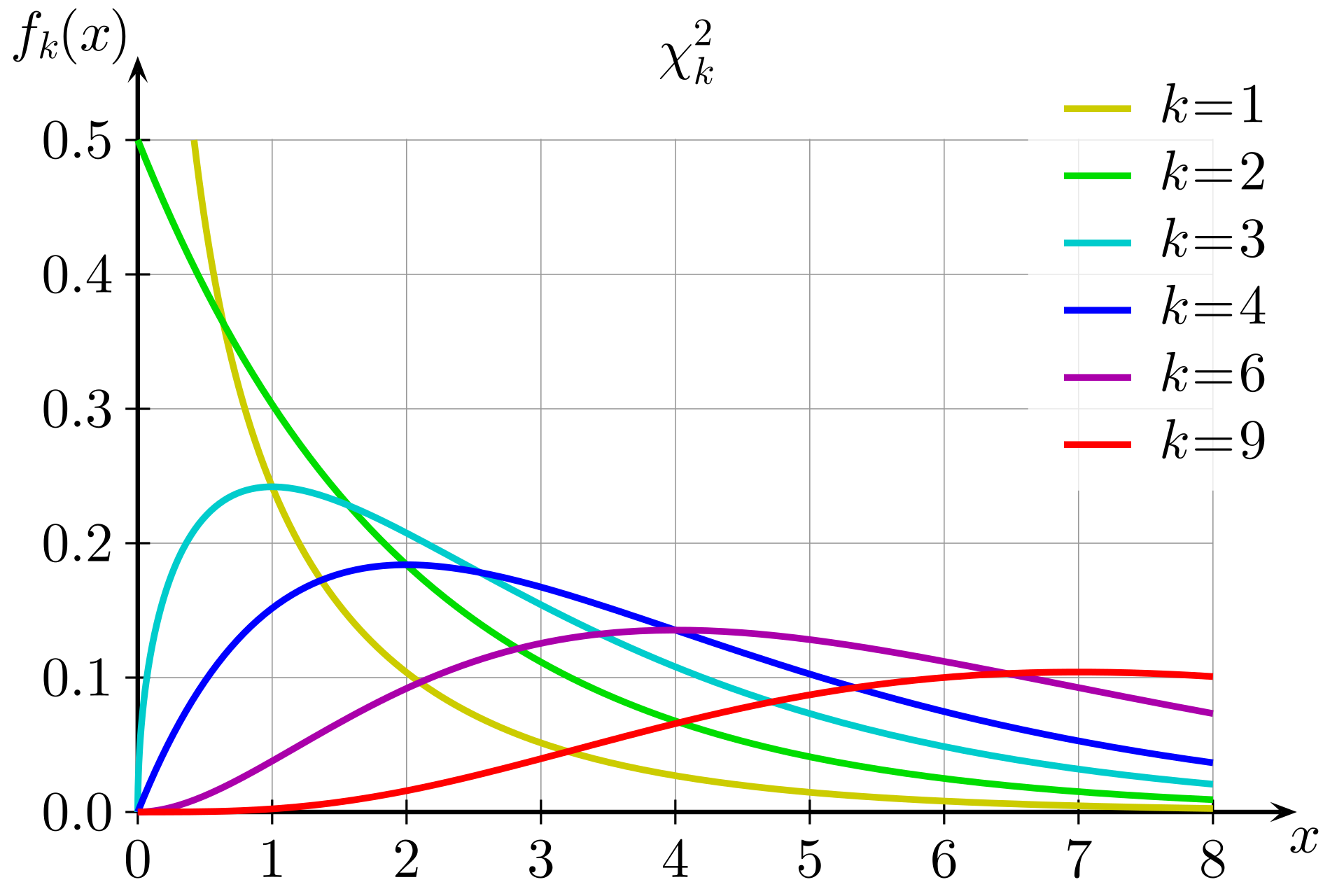
This is the probability frequency distribution of the $\chi^2$ distribution. It is defined by one parameter, $k$, which represents the number of summed independent squared standard normal variables. In the applied setting, $k$ is equal to the degrees of freedom in your model.
On this plot, \(x=Z_1^2+Z^2_2+{...}+Z^2_k.\)
We can use the visual example to supplement our intuition. For $k=1$ (the yellow line), the modal value seems to be around $0$. This aligns with our previous expectations: the modal value for a squared standard normal variable is $0$. As the number of variables increases, the modal value shifts to the right. This makes sense, because more variables means it’s less likely that they all sum to $0$. Formally, the modal value is defined as the max of $(0, k-2)$.
Because the values of the $Z$ variables are squared, the $\chi^2$ distribution is purely non-negative. It has the property that the mean is $k$ while the variance is $2k$.
Pearson’s chi-squared test
A goodness-of-fit test is a test that compares observed data to an expected distribution.
Many times in psych research, we have data that are categorical, not continuous. Common examples are: biological sex, marital status, type of therapy/treatment, etc. When we want to test if our observed data were due to chance, we can use a specific goodness-of-fit test: a chi-square ($\chi^2$) test. This is a nonparametric test which compares the observed frequency distribution of a categorical variable to the expected frequency distribution.
To learn about the $\chi^2$ test, we’ll use an applied example. Imagine that you survey 99 people on their favorite first-generation starter Pokémon. You get data that are summarized in the table below:
| Bulbasaur | Charmander | Squirtle |
|---|---|---|
| 21 | 59 | 19 |
We want to test if there is a systematic element to these data, or if they were simply due to chance. To do so, we calculate a test statistic and compare it to a null hypothesis. The null hypothesis for the $\chi^2$ test is that the data in each category follow a specific set of probabilities. In our case this corresponds to an equal number of observations for each category in the population. Because this test is nonparametric, we do not estimate a point estimate of the proportions in each category, and do not describe population parameters mathematically. Rather, we get a single test statistic that corresponds to a p-value: the probability of getting results as or more extreme as the observed results, assuming the null hypothesis is true. Our alternative hypothesis is that some systematic difference does exist in the population between our categories.
$H_0:$ All categories have the same frequency in the population.
$H_1:$ Not $H_0$.
The $\chi^2$ statistic is defined as $\chi^2=\sum_i \frac{(O_i-E)^2}{E}$ where $O_1, O_2, {…}, O_i$ are the observed frequencies for our categories, and $E$ is the expected frequency. The expected frequency is calculated as $E = \frac{N}{i}$ where $i$ is the number of categories in our data.
So, for our Pokémon example, we can calculate the expected value as $E = \frac{99}{3}=33$, so we expect to observe $33$ people in each condition, if $H_0$. We can then calculate our $\chi^2$ as $\chi^2=\sum_i \frac{(O_i-E)^2}{E}=\frac{(21-33)^2}{33}+\frac{(59-33)^2}{33}+\frac{(19-33)^2}{33}=30.79$.
Now that we have our test statistic, we need to compare it to a critical value. We can look up the critical value from a chi-square table with our given degrees of freedom. For the single variable case, the degrees of freedom is calculated as $df=i-1$ where $i$ is the number of categories in our data. This is because, for a given $N$, the final category frequency cannot vary after the other two have been established. So, the degrees of freedom for our example is $2$.

From the table, we can see that the critical value at $p=.05$ for two degrees of freedom is $\chi^2_{crit}=5.991$. Because our test statistic is greater in magnitude than our critical value, we reject the null hypothesis and conclude that there is a significant difference in category frequencies in our data. Importantly, it does not tell us where exactly the distinction lies. We cannot make any more specific claims than the fact that the frequency proportions are unequal.
The chi-square test of independence
Often, we may also want to compare the frequencies of two categorical variables to each other in order to determine if they are independent. For example, if we have data concerning someone’s favorite genre of movie by biological sex, it might take the following form:
| Horror | Action | Comedy | Row Total | |
|---|---|---|---|---|
| Male | 15 | 45 | 30 | 90 |
| Female | 35 | 20 | 30 | 85 |
| Column Total | 50 | 65 | 60 | 175 |
This is known as a contingency table: the frequencies of one variable contingent upon the other.
The $\chi^2$ statistic is calculated exactly the same way as before, with one important caveat. Now, the expected value for each cell is determined by the formula $E(r,c)=\frac{N(r) \cdot N(c)}{N}$ where $N$ is the total number of observations, $r$ is the row total, and $c$ is the column total. The logic for this formula is that we want to calculate the expected proportion of data in a cell, given the row and column totals. For each cell, the expected proportion can be found by multiplying the two row and column proportions together: $\frac{r}{N} \cdot \frac{c}{N} = \frac{rc}{N^2}$. Multiplying again by $N$ rescales it to be the overall expected proportion in the cell. So, our expected cell values are conditional on the row and column totals. This is what we want. If one column total is simply more frequent in the population, we want to determine if it has an effect across our other variable above and beyond its simple popularity. Considering row and column totals allows us to test for independence.
In this example, our chi-square statistic can be calculated as $\chi^2=\sum_j^k \sum_i^h \frac{(O_{ij}-E_{ij})^2}{E_{ij}}$ where one variable has $k$ levels and the other has $h$ levels.
\[\chi^2=\sum_j^k \sum_i^h \frac{(O_{ij}-E_{ij})^2}{E_{ij}}=f \chi^2=\frac{(15-25.71)^2}{25.71}+\] \[\frac{(45-33.43)^2}{33.43}+\frac{(30-30.86)^2}{30.86}+\] \[\frac{(35-24.29)^2}{24.29}+\frac{(20-31.57)^2}{31.57}+\frac{(30-29.14)^2}{29.14}\] \[=17.49\]The degrees of freedom can be calculated the same way, except we subtract $1$ from the levels of categories in each group: $df=(h-1)(k-1)=(2-1)(3-1)=2$. So, our critical value is the same as in the previous example: $\chi^2_{crit}=5.991$. Because our observed $\chi^2$ statistic is greater than the critical value, we once again reject the null hypothesis and conclude that there is a statistically significant relationship between our two nominal variables.
Relationship between chi-square distribution and test
By now, you may be wondering how these tests are weighed against the chi-square distribution. After all, the distribution was introduced as the resulting distribution when you sum squared independent standard variables. How does it connect?
When you have a contingency table, the data in each cell is assumed Poisson, meaning that the probability distribution is modeled by the number of occurrences (frequency) expected in a specific interval (row/column totals). A Poisson distribution has mean and variance equal to its singular parameter $\lambda$, and in the contingency table $\lambda_{ij}$ is assumed to equal $E_{ij}$. Thus, standardizing the observations in each cell gives $\frac{O_{ij}-E_{ij}}{\sqrt(E_{ij})}$. If these standardized values are summed and squared, we get exactly the chi-square formula: $\sum_j^k \sum_i^h \frac{(O_{ij}-E_{ij})^2}{E_{ij}}$. The Poisson distribution asymptotically approximates a normal distribution, so this formula asymptotically approximates a chi-square distribution.
Model fit information
In structural equation models, model fit is often conceptualized as how well the model-implied covariance matrix matches the sample data covariance matrix. According to Jöreskog, 1969, the log-likelihood function for a model is given by $F(\Lambda, \Phi, \Psi)=log \lvert \Sigma \rvert + tr(S \Sigma^{-1}) - log \lvert S \rvert -p$. When this function is minimized, $n$ times the resulting value is equal to the chi-square distributed likelihood ratio test statistic of goodness of fit. What this means is that one common model fit statistic is chi-square distributed.
Of course, this statistic has been criticized for being overly sensitive to sample size. Because the $F$ value is multiplied by $n$, large sample sizes will almost always be significant, even for arbitrary deviations from chi-square.
Conclusions
The $\chi^2$ distribution is often encountered quite early in statistical training, but not fully explored (especially in the field of psychology). Thus, when students encounter statements such as “the difference between likelihoods of nested models follows a $\chi^2$ distribution,” they may not have the best intuitive understanding of what this means. I hope this brief overview has been helpful.