Grad School Scramble III: Inter-rater Reliability

Well, here we are! Summer is over, the new students are flocking to campus, and I find myself in the beautiful and hot state of Arizona. Classes technically started on Thursday, but they mostly consisted of looking over syllabi and introducing yourself to your classmates. The ASU program is great so far: my fellow grad students are awesome, the faculty are trememdous, and I’ve already begun immersing myself in local communities like choir and card shops.

During one of my Friday classes, Professional Issues in Psychology (or, as it’s informally known, Intro to Being a Grad Student), the instructor Cheryl Conrad told an anecdotal story about inter-rater reliability. As she was telling it, I realized that I really don’t know much about the concept, and decided that it would be a good installment of Grad School Scramble. I have not been nearly as prolific with this series as I had hoped, but I wanted to finish one last post before school gets heavily underway. Who knows—maybe I’ll continue it into the semester.

Inter-rater reliability: Definitions and concepts

Psychological studies and tests can often require responses that are long, involved, or otherwise unable to be directly assessed numerically. When such responses are present in a test, they are often interpreted by an individual (or individuals) to convert them to a format that can be analyzed. For example, essays on AP exams are sent to independent readers that rate the essays on a scale from 0-6. In AP’s case, two independent readers will score each essay, so that an individual score isn’t biased by one single reader. For more general tests and studies, these readers are generally known as “raters,” and it’s critically important that they are accurately and reliably assessing each response.

How can we determine if raters are doing a good job? One method is by evaluating the inter-rater reliability: a measure of how much the raters are agreeing with each other. If they display a large amount of agreement, we have reason to believe that their judgments are valid; conversely, if they disagree frequently, there might be reason to doubt the validity of their ratings. With that said, how do we measure their agreement?

Before diving into agreement measures, it’s important to discuss what we even mean by “agreement.” When scoring is categorical, agreement is simple: the raters either agree or they don’t. When scoring is ordinal or better, however, the question of “scoring distance” comes into play. Raters who score an essay 5 and 6 respectively seem to agree more than raters who score an essay 1 and 6, but they still disagreed. How do we account for that? Furthermore, there are different types of rating. There exists the aforementioned scoring where raters are agreeing/disagreeing with a single rating, but what about if they’re both confirming an official score? What if they’re ranking different options? What if there are more than 2 raters? There are a variety of different measures to quantify agreement in each of these situations.

Simple probability of agreement

The first and easiest example of an agreement measure is the probability of agreement. This measure is only applicable for nominal data, but it was the standard method of determining inter-rater reliability for a lengthy era of quantitative methodology. When there are 2 or more raters scoring a response, it is easy to calculate the percentage of the time that they agree. We simply divide the number of identical scores by the total number of scores and obtain the percent agreement. When there are more than two raters, we can set up a matrix in which each row represents a variable of interest and each column is a rater score.

According to McHugh (2012) (who I shamelessly stole the matrix example from), the direct interpretation of the probability of agreement is the percent of valid data. That is, if you have 90% percent agreement, then 10% of the data in your study are erroneous.

Cohen’s kappa

As we can see from the previous example, the joint probability of agreement has some issues as a measure of inter-rater reliability. For one, it is only applicable for nominal data. Furthermore, its interpretation is overly simplistic and doesn’t tell you much about the direction of erroneous data. The biggest issue, however, is the one that statistician Jacob Cohen pointed out in the ’60s: it doesn’t account for agreement that arises due to chance. For example, if two professors were to rate student performance on a test as either pass/fail, and we asked them to give scores completely randomly, we would still expect them to coincidentally give the same rating about half of the time. On paper, they would seem to exhibit 50% congruence, but in reality there would be no systematic agreement between the two raters.

To account for this, Cohen developed Cohen’s kappa, stylized as $\kappa$, as a correlational coefficient of rater agreement. It ranges from $-1$ to $1$, with $-1$ representing perfect disagreement, $1$ representing perfect agreement, and $0$ representing the agreement we would expect due to random chance.

The formula is as follows:

$\kappa=\frac{p_o-p_e}{1-p_e}$

where $p_o$ is the observed percent agreement and $p_e$ is the expected percent agreement due to chance.

The intuition behind the formula is that $p_o-p_e$ represents subtracting the expected chance percentage of agreement from the observed percentage, leaving the “non-chance” percentage of agreement left. Dividing by $1-p_e$ rescales the result so that $1$ is perfect agreement and $0$ is random chance. For example, if you expect 50% of your agreement to be due to chance and your raters perfectly agree, then you would still get a kappa coefficient of $1=\frac{1-.5}{1-.5}$. If you expected 50% of your agreement to be due to chance and your raters agreed 50% of the time, then you would get a kappa coefficient of $0=\frac{.5-.5}{1-.5}$.

For 2 raters, $p_e$ can be calculated by a chi-square table where each class is a rater. For example:

If this is our chi-square table (forgive the poor $ \LaTeX $), and rater 1 is the columns (rating of pass/fail) while rater 2 is the rows (rating of pass/fail), then we can calculate the expected agreement due to chance as follows. We can find the sum total of each row and column as $112$ and $93$ for the rows, and $103$ and $102$ for the columns, respectively. The total $n$ of the ratings is 205. According to the rule of independent probability, if our data were all independent then knowing the row tells you nothing about which column some data might be in. Let’s take the example of the top-left cell, which is the intersection of row 1 and column 1. Formally, if $P(A)$ is the probability that a variable is in row 1 and $P(B)$ is the probability that a variable is in column 1, then $P(A\space and\space B)=P(A)\cdot P(B)$. By the definition of a chi-square table, $P(A)=\frac{100+12}{205}=0.55$ and $P(B)=\frac{100+3}{205}=0.50$. Thus, $P(A)\cdot P(B)=.28$. So, if all of our data were due to random chance we would expect the top-left-most cell to contain 28% of our data, or a total of about 57. We can repeat this process for the other cells and sum up the totals of the congruent cells to determine the percent agreement we would expect due to chance. At the end of this process, it turns out that this chi-square table results in a $p_e=.50$, which is an expected percentage of agreement due to chance around 50% of the time. (For more information on probability, feel free to read my blog post about basic concepts in probability)

Circling back to Cohen’s kappa: Once we know the expected probability $p_e$, we can finish our formula. Our total agreement $p_o$ is $\frac{190}{205}\approx.93$. When we substitute these numbers back into our kappa formula we get $\kappa=\frac{p_o-p_e}{1-p_e}=\frac{.93-.50}{1-.50}=0.85$.

Can anyone see an issue with Cohen’s kappa from this example? I have one: It makes the assumption that ratings due to chance would follow the distribution of rows and columns exactly equal to the numbers we observe. Due to this, Cohen’s kappa can sometimes be too critical of inter-rater reliability because it assumes that random chance ratings would look similar to the marginal proportions observed. It also assumes that raters are always independent. Despite this, $\kappa$ remains a more robust estimation of rater agreement than percent agreement.

Because $\kappa$ is a correlation coefficient, it cannot be directly interpreted.

Quick note: while I was researching and reading stuff for this post, I came across the aforementioned McHugh (2012) paper which stated that squaring kappa results in the “amount of accuracy” due to agreement between the raters. This is a foundational article, with almost 22,000 citations. Regardless, I could not find any information to back this idea up, and plugging some example numbers into a quick Cohen’s kappa calculator seemed to disprove it. Their justification was that squaring any correlation coefficient results in an estimate of the variance explained, but I am not knowledgeable enough to confirm nor deny this. Can anyone smarter than me chime in and help with this?

Regardless of the interpretation of kappa squared, we have accurate and verifiable standards for Cohen’s kappa. The following table shows which values are deemed acceptable:

Weighted Cohen’s kappa

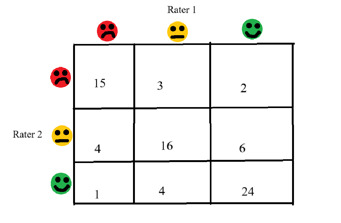
In situations where raters need to make ordinal scorings with more than 2 categories—such as ranking patient pain from mild/moderate/severe—Cohen’s kappa has another issue: It does not differentiate between “levels” of disagreement. In the example of patient pain, we might want to quantify the disagreement between a doctor recording “mild pain” and a second doctor recording “severe pain” as a more extreme disagreement than “mild pain” and “moderate pain.” However, if we set up our 3x3 contingency table and calculate the expected percentages of agreement/disagreement, all disagreements are weighted equally.

To solve this problem, in 1968 Cohen published an extension to kappa known as weighted kappa (although, arguably, normal kappa is a special extension of weighted kappa). Using weighted kappa allows for a researcher to assign weights to disagreements such that some can be viewed as more extreme than others.

How does it work? Well, the formula for weighted kappa is as follows:

$\kappa _w{}=1-\frac{\Sigma v_{ij}p_{oij}}{\Sigma v_{ij}p_{eij}}$

To obtain this formula, Cohen began with some simple algebra from the formula for $\kappa$. As a reminder,

$\kappa=\frac{p_o-p_e}{1-p_e}$.

If we let $q$ represent the proportion of disagreement and define $q=1-p$, then we can do the following algebra:
$q+p=1$,
$p=1-q$.

From here, we can represent our observed agreement and expected agreement in terms of $q$:
$p_o=1-q_o$,
$p_e=1-q_e$.

Now, we can substitute these values into the original formula for $\kappa$:

$\kappa=\frac{p_o-p_e}{1-p_e}=\frac{(1-q_0)-(1-q_e)}{1-(1-q_e)}$.

After some simple algebra, we get $\kappa=\frac{q_e-q_o}{q_e}$. If we then divide both sides of the fraction by $q_e$, we get $\frac{1-\frac{q_o}{q_e}}{1}$, which quickly simplifies to:

$\kappa=1-\frac{q_o}{q_e}$.

Now we have our original kappa formula in terms of the proportion of disagreement between the raters. Cohen next introduces a weighting concept based on the strength of disagreements. If we imagine a contingency table set up as so:

Then we want to weight the disagreements so that more severe disagreements are more costly to $\kappa$. The way in which this is done is up to the researcher; but, as Cohen stresses, it must be done prior to the collection of data. One common weighting method is linear weighting, where the weight assigned to each disagreement is simply the distance between the two cells:

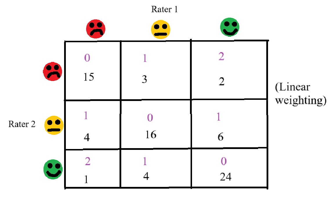
The weights are the numbers in purple

Another alternative is to use quadratic weighting, which is when the distance between the incongruent cells is squared. Finally, as can be shown algebraically, when all disagreeing cells are weighted equally it recovers the original definition of $\kappa$.

$\kappa{_w}$ simply represents the original kappa formula with $p_o$ and $p_e$ replaced by weighted proportions of disagreement. So, for each cell, we multiply the proportion (or frequency) by the weight, and get our weighted proportion. When we add this weighting factor back into our modified kappa formula we get the final $\kappa{_w}$ formula, which is:

$\kappa _w=1-\frac{\Sigma v_{ij}p_{oij}}{\Sigma v_{ij}p_{eij}}$

where $v_{ij}$ represents the weighting factor for cell $i,j$.

Finally, we want to prove that this recovers the original kappa formula when all weights are equal. If we assume that all cells are weighted equally, then $v_{ij}$ becomes some non-zero constant, which can then be pulled out of the summation. After that, the constant can be cancelled out of the numerator and denominator, giving the formula:

$\kappa _w=1-\frac{p_{oij}}{p_{eij}}$,

which can be understood as our original kappa proportion of disagreement.

For the purposes of space and time, I won’t be going through a full hand-calculated example of weighted kappa, but I hope that this run-through of the formulae was enough to serve as a decent introduction.

Pearson’s r

If ratings are continuous, then Pearson’s r can be used pairwise as a measure of inter-rater reliability. However, this is mostly a poor choice, because it fails to take into account systematic biases between the two raters. For example, if one rater scores a measure (1, 2, 3, 4, 5) while another rater scores pairwise the same measure (2, 3, 4, 5, 6), then their correlation will be 1, but there will be difference in their agreement. So, I’m not going to go very in-depth into the usage of r as a measure of inter-rater reliability. Just know that it’s technically an option.

Intraclass Correlation Coefficient

So, what should we use if ratings are continuous (interval or ratio)? One option is to use the Intraclass Correlation Coefficient (ICC). From a mixed-models standpoint (as was explained to me by the amazing Catherine Bain), the ICC is the amount of variance of the intercepts divided by the total variance (which comprises the variance of the intercepts + the unwanted variance). So, if the unwanted variance is higher than the variance of the intercepts, then the ICC is lower than $.5$ (which is a poor result). On the other hand, if the variance of the intercepts composes a large amount of the variance than the ICC will be higher.

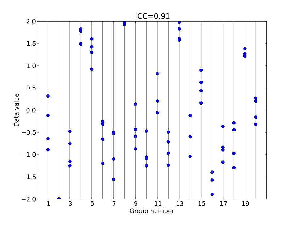
We can extend this idea to inter-rater reliability by considering the items as the clusters and determining how much variance in score is due to item difference vs. rater difference. If we look at the previous chart, if we let “Group Number” represent the different items and the blue dots represent the scores that raters assign to the item, then we can observe how the individual item is much more predictive of a score than the distinctive rater. This is what we want to see—and displays a good ICC of $.91$. Conversely, if there was more of a difference between raters than between items, then there would be more “unwanted variance” than intercept variance, and the ICC would be much lower.

Unlike Cohen’s kappa, the ICC compares to a theoretical null model of “no intercept variance” which is more straightforward than the kappa assumption about what chance agreement would look like. This can make it more useful under certain conditions. However, according to Wikipedia the ICC does make the assumption that raters are exchangable for a certain item. In other words, there is no meaningful way to order the raters. This assumption is violated if there is systematic bias between different raters (which would result in some raters being naturally more critical than others), which is likely in real-world scenarios, so debate exists about whether other measures should still be used in place of the ICC.

As always, I am not a professional, so I feel the need to give the disclaimer that I don’t have a full mathematical understanding of how the ICC works. Nor do I have an understanding of mixed models past what you can get from a couple of YouTube videos. Still, I hope that most of the information presented is at least somewhat accurate.

Concluding thoughts

Well, there you have it. The results of 3 days of reading information about inter-rater reliability. Is it super, incredibly useful? I’m not sure—I’ve never been a part of a study with multiple raters. In any case, it certainly was interesting. One of my big take-aways is how amazing Jacob Cohen’s work was, especially for the time. I learned about kappa before investigating weighted kappa, and the weighted version seemed a very powerful yet natural extension of the previous work. I tried for almost an hour to sit down and derive the formlua for weighted kappa from the unweighted version, and couldn’t figure it out (even with the weighted formula sitting in front of me). Lo and behold, Cohen does it in like three lines on the third page of his paper. Sometimes it almost feels like we’re falling off the shoulders of giants.